Upper Missouri River Basin Soil Moisture and Snowpack Dashboard
NOAA’s National Integrated Drought Information System (NIDIS) and National Centers for Environmental Information (NCEI), Montana Mesonet, Nebraska Mesonet, Mesonet at South Dakota State University, North Dakota Agricultural Weather Network (NDAWN), Wyoming Mesonet, U.S. Army Corps of Engineers
Note: This dashboard is experimental. Please read all map descriptions carefully.
Under Congressional direction, NOAA's National Integrated Drought Information System (NIDIS) is leading the Upper Missouri River Basin Data Value Study, an interagency study of the value of the data from the Upper Missouri River Basin Soil Moisture and Plains Snow Monitoring Build-Out to support improvements to water resource models, drought monitoring capabilities, and other applications. One goal of this study is to produce publicly-available, basin-wide soil moisture and snowpack data and maps on Drought.gov to support the U.S. Drought Monitor authors and contributors.
To facilitate access to the diverse datasets necessary to fully monitor basin-wide hydrological conditions, the U.S. Drought Portal team created an interactive dashboard. The Drought Portal team ingests station-based soil moisture and snowpack data from the five state mesonets in the Upper Missouri River Basin (UMRB)—Montana, Nebraska, North Dakota, South Dakota, and Wyoming. Data are ingested via Synoptic, who is contracted by the National Weather Service’s National Mesonet Program to develop the UMRB data access platform. Soil moisture and snowpack data are valid through 12z each Tuesday, and are displayed in actionable maps. Overlays, such as the U.S. Drought Monitor or snow water equivalent (SWE), are also available to provide additional context to station-level observations that inform drought monitoring and decision-making in the region.
Available maps include:
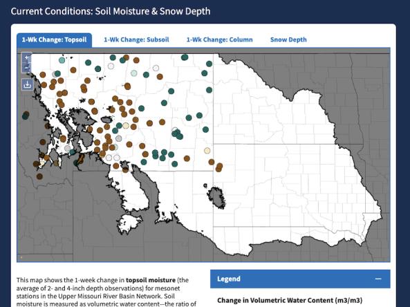
- Soil moisture (volumetric water content) change maps for 1, 4, 8, and 12 weeks, which can show important trends in evolving conditions
- Fractional available water (FAW), shown as a percentage from 0%–100%
- Categorized soil moisture
- Snow depth current conditions (inches).
All soil moisture maps are available for three soil layers:
- Topsoil: Average of 2- and 4-inch depth observations
- Subsoil: Average of 8- and 20-inch depth observations
- Total Column: Average of 2-, 4-, 8-, and 20-inch depth observations.
Additional maps, such as frost and thaw depth, are planned for future phases of development. Because of the current short period of record for this new network, volumetric water content anomalies or percentiles are not yet available.
For additional soil moisture and snowpack data and information, visit the five UMRB state mesonets, or view time series graphs of the data on the U.S. Army Corps of Engineers UMRB Monitoring Network page.
Fractional available water (or FAW) is the amount of water in the soil available for plant use. Specifically, FAW is the ratio of currently available water divided by the available water at capacity. Therefore, this measure approaches zero as moisture available to plants from the soil decreases, which can be an indicator of drought conditions.
On this map, available water for the total column (2-, 4-, 8-, and 20-inch depths) is shown as a percentage, where 0% is the wilting point (the soil moisture content at which plants have limited access to moisture) and 100% is the field capacity (the amount of water the soil can hold). Learn more about this map.
Categorized soil moisture groups current soil moisture conditions into one of four categories based on the vegetation’s level of access to that moisture. This map shows categorized soil moisture for the total column (2-, 4-, 8-, and 20-inch depths).
Very Short (orange) conditions occur when soil moisture is below the wilting point, the point at which plants begin to wilt and (over time) fail to recover. Short (yellow) means that soil moisture is still limited but not as severely (above wilting point). Adequate (green) represents ideal conditions for vegetation’s access to soil moisture, and Surplus (blue) means that moisture exceeds the holding capacity (field capacity) of the soil.
This metric can be useful in identifying where and when vegetation may be stressed as a result of prolonged exposure to drought, which is an important aspect of drought monitoring and assessment. Learn more about this map.
Soil moisture plays an important role in drought and flood forecasting, agricultural monitoring, forest fire prediction, water supply management, and other natural resource activities. Soil moisture observations can forewarn of impending drought or flood conditions before other more standard indicators are triggered.
Learn MoreDrought can result in reduced growth rates, increased stress on vegetation, and alterations or transformations to the plant community and/or the entire ecosystem. During periods of drought, plants increase their demand for water through increased evapotranspiration and longer growing seasons.
Learn MoreSoil moisture plays an important role in drought and flood forecasting, agricultural monitoring, forest fire prediction, water supply management, and other natural resource activities. Soil moisture observations can forewarn of impending drought or flood conditions before other more standard indicators are triggered.
Learn MoreDrought can result in reduced growth rates, increased stress on vegetation, and alterations or transformations to the plant community and/or the entire ecosystem. During periods of drought, plants increase their demand for water through increased evapotranspiration and longer growing seasons.
Learn MoreFractional Available Water (%)
No Data
No data are available for this station.
Category
Very Short
Short
Adequate
Surplus
No Data
Fractional available water (or FAW) is the amount of water in the soil available for plant use. Specifically, FAW is the ratio of currently available water divided by the available water at capacity. Therefore, this measure approaches zero as moisture available to plants from the soil decreases, which can be an indicator of drought conditions.
On this map, available water for the total column (2-, 4-, 8-, and 20-inch depths) is shown as a percentage, where 0% is the wilting point (the soil moisture content at which plants have limited access to moisture) and 100% is the field capacity (the amount of water the soil can hold). Learn more about this map.
Categorized soil moisture groups current soil moisture conditions into one of four categories based on the vegetation’s level of access to that moisture. This map shows categorized soil moisture for the total column (2-, 4-, 8-, and 20-inch depths).
Very Short (orange) conditions occur when soil moisture is below the wilting point, the point at which plants begin to wilt and (over time) fail to recover. Short (yellow) means that soil moisture is still limited but not as severely (above wilting point). Adequate (green) represents ideal conditions for vegetation’s access to soil moisture, and Surplus (blue) means that moisture exceeds the holding capacity (field capacity) of the soil.
This metric can be useful in identifying where and when vegetation may be stressed as a result of prolonged exposure to drought, which is an important aspect of drought monitoring and assessment. Learn more about this map.
These fractional available water (FAW) maps update weekly, with data valid through Tuesday at 12Z (7 a.m. ET).
These categorized soil moisture maps update weekly, with data valid through Tuesday at 12Z (7 a.m. ET).
Soil moisture plays an important role in drought and flood forecasting, agricultural monitoring, forest fire prediction, water supply management, and other natural resource activities. Soil moisture observations can forewarn of impending drought or flood conditions before other more standard indicators are triggered.
Learn MoreDrought can result in reduced growth rates, increased stress on vegetation, and alterations or transformations to the plant community and/or the entire ecosystem. During periods of drought, plants increase their demand for water through increased evapotranspiration and longer growing seasons.
Learn MoreSoil moisture plays an important role in drought and flood forecasting, agricultural monitoring, forest fire prediction, water supply management, and other natural resource activities. Soil moisture observations can forewarn of impending drought or flood conditions before other more standard indicators are triggered.
Learn MoreDrought can result in reduced growth rates, increased stress on vegetation, and alterations or transformations to the plant community and/or the entire ecosystem. During periods of drought, plants increase their demand for water through increased evapotranspiration and longer growing seasons.
Learn MoreAccess
UMRB Soil Moisture & Snowpack Dashboard
UMRB Monitoring Network Data: View and download time series graphs of soil moisture and snow data, as well as photos of the mesonet stations.
View soil moisture and snowpack data from the UMRB state mesonets:
Soil Moisture Change Map Methodology
Weekly changes in soil moisture conditions provide one of the most straightforward measures of evolving or trending hydrological conditions. To represent a variety of short- to long-term conditions, weekly changes in volumetric water content (VWC) are represented in units of m3/m3 for topsoil (2-inch and 4-inch depth observations), subsoil (8-inch and 20-inch depth observations), and column (2-, 4-, 8-, and 20-inch depth observations). Differences are computed as the most recent Tuesday at 12Z minus Tuesday at 12Z X weeks ago.
Computing Change Maps with Frozen Soils
The type of soil moisture sensors deployed across the Upper Missouri River Basin and at most monitoring networks are not well suited to quantify ice water content, which complicates efforts to derive soil moisture change around the winter season. However, ice water content is generally unaffected by hydrological processes (i.e., gravitation drainage, lateral or downhill flow, or evapotranspiration) such that it can be well approximated by liquid water content immediately following pre-freeze. A general consensus based on feedback from soil scientists and leading experts in this field has identified that soil temperatures at or above 2°C have near negligible ice water content. Given the stasis of ice water content, it is reasonable to compute a soil moisture change when one or both ends of the change period are in a frozen condition by substituting the most recent unfrozen (soil temperature > 2°C) soil moisture observation. Stations with shifted dates due to frozen soil conditions are denoted with a triangle on the soil moisture change maps.
Soil Moisture Change Plots
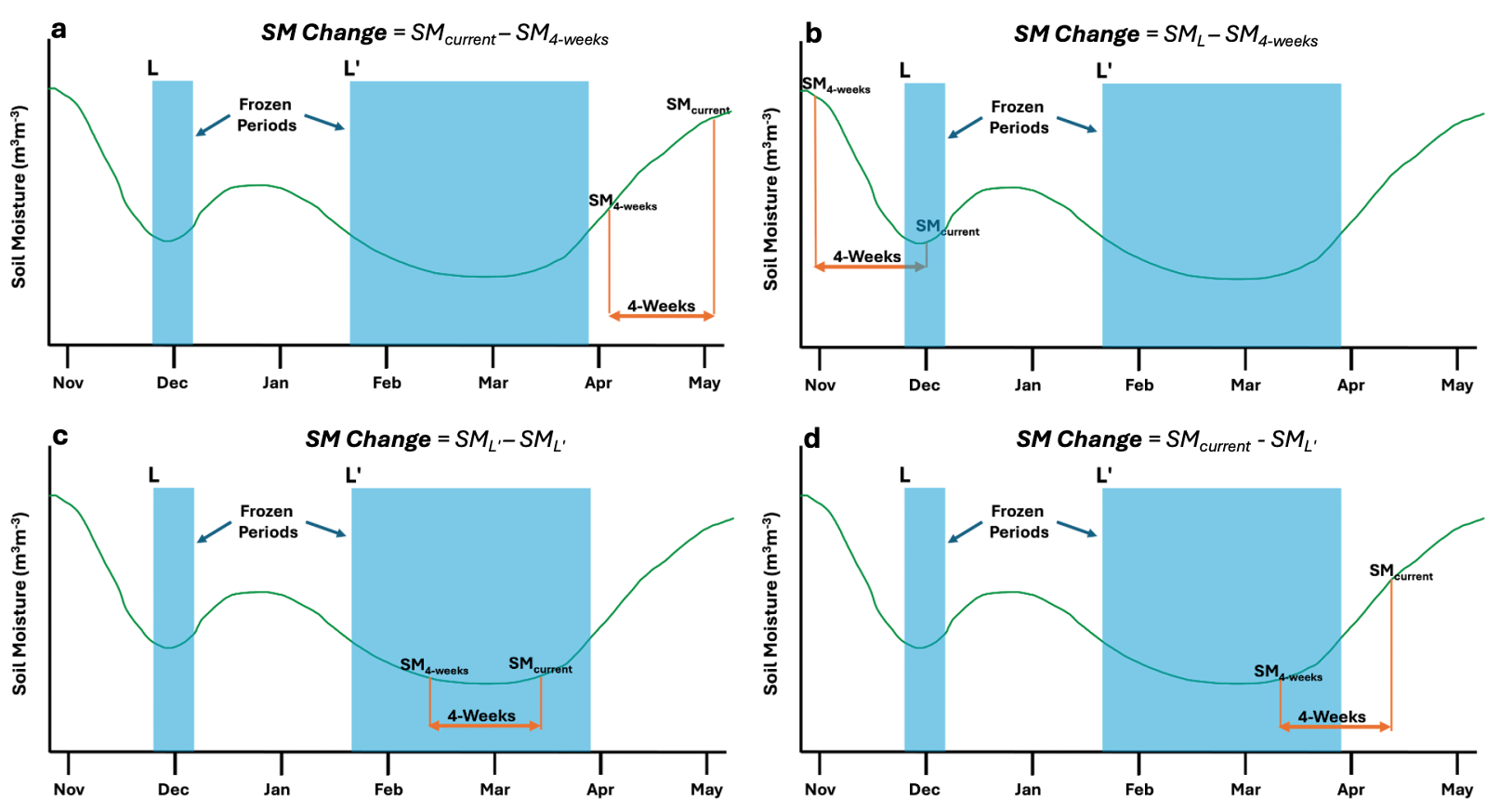
To compute soil moisture change, valid observations of both soil moisture and temperature are necessary. Differences are to be computed at each depth individually as current Tuesday at 12Z (SMcurrent) minus starting Tuesday at 12Z X-weeks ago (SMx-weeks). For instance, a 4-week soil moisture change is SMcurrent minus SM4-weeks (Fig 1a). Soil moisture change at each depth is then averaged over the respective layer's (i.e., top, subsoil, column) depths.
To derive a soil moisture change for a period, set i to the current Tuesday at 12Z representing SMcurrent.
- If soil temperature at week i (STi) is missing then set SMcurrent to missing.
- If soil moisture at week i (SMi) is missing and STi ≥ 2°C, then set SMcurrent to missing.
- If STi > 2°C then set SMcurrent to SMi.
- If STi is less than < 2°C then set i to the previous week (i-1) and repeat this process until one finds an observation week in the past where STi > 2°C. Then, set SMcurrent to SMi
This same process will be used to define SMx-weeks with i initially set to the respective Tuesday at 12Z X-weeks ago.
In this way, changes in soil moisture that temporally include frozen soils represent the liquid water content change over that period (Fig. 1). For a 4-week change map, SMcurrent and SM4-week will represent soil moisture conditions based on soil temperature for Fig. 1.
- When STcurrent ≥ 2°C and STx-weeks ≥ 2°C (outside of frozen period), SMcurrent and SM4-week represented the soil moisture conditions for the current Tuesday and Tuesday 4 weeks ago at 12Z (Fig. 1a). SMChange = SMcurrent – SM4-weeks
- When STcurrent < 2°C and ST4-weeks ≥ 2°C (going into a frozen period) SMcurrent will be set to the soil moisture value on the Tuesday at 12Z denoted by L (SML) as noted in (Fig. 1b).
- When STcurrent < 2°C and ST4-weeks < 2°C (contained in frozen period) SMcurrent and SMx-weeks are both set to the Tuesday at 12Z denoted by L` (SML`), which represents no change (Fig. 1c).
- When STcurrent ≥ 2°C and STx-weeks < 2°C (emerging from frozen period), SM4-weeks is set to the Tuesday at 12Z denoted by L` (SML`) as shown in Fig. 1d.
Fractional Available Water (FAW) Methodology
Fractional available water (or FAW) is a measure of the amount of moisture in the soil available to plants. Since this measure is sensitive to soil type (e.g., density, texture), FAW is a useful metric that accounts for differences in soil properties across diverse regions and a useful metric for agricultural drought. FAW values are typically represented as a fraction; however, for this product we are displaying them as a percentage ranging from 0% (limited available water) to 100% (plenty of available water). It is possible to exceed 100% during heavy rains and dip below 0% during droughts, but values above 100% and below 0% were capped at the respective 100% and 0% levels. This was done since values below 0% do not necessarily change the interpretation that water available to plants is limited; this is also the case for values above 100%.
FAW is computed as a ratio of the current available water to plants (AvailableWater) divided by soil water capacity (WaterCapacity; see eq. 1). These quantities are based on two critical thresholds that describe the lower and upper limits of soil moisture available to plants, referred to as the wilting point (WP) and field capacity (FC), respectively. Moisture in the soil at and below WP would require capillary pressures beyond the capacity of most vegetation (-1,500 kPa) to extract additional moisture from the soil. During heavy precipitation events, soil moisture conditions can exceed FC such that the additional moisture will be quickly drained (to deeper depths or horizontally) before plants can access that moisture and is therefore unavailable to the plant as well. Given these conditions, AvailableWater is defined as the current soil moisture observation at UMRB mesonet stations (ObsSM) minus WP (eq. 2) with WaterCapacity derived as FC minus WP (eq. 3). As a result, FAW is computed as shown in equation 4.
FAW = AvailableWater / WaterCapacity (eq. 1)
AvailableWater = ObsSM - WP (eq. 2)
WaterCapacity = FC - WP (eq. 3)
FAW = (ObsSM - WP)/(FC - WP) (eq. 4)
The WP and FC thresholds were defined for each station depth using a combination of soil property information from USDA’s gNATSGO database (i.e., percentages of sand, silt, and clay) to drive the Rosetta version 3 model. This model estimates the van Genuchten parameters allowing one to build a water retention curve for each station depth. The station depth’s WP and

FC were extracted along this curve at -1,500 kPa (WP) and -33 (FC) kPa, respectively. For station depths that had over 52% sand or a combination of higher percentages of sand (~42% or more) and silt (~28% or more), the -10 kPa threshold was used to define FC.
Layer composites (e.g., topsoil, subsoil) of FAW were derived as the sum of the 24-hour averaged AvailableWater ending Tuesday at 12Z for each depth in the layer divided by the sum of the WaterCapacity over each depth in that layer. For instance, topsoil FAW is computed as the sum of the 2-inch and 4-inch depths’ hourly (h) averaged AvailableWater observations, divided by the sum of their respective WaterCapacities. This process is repeated for the subsoil (8-inch and 20-inch) and column (2-inch, 4-inch, 8-inch, and 20-inch) layers, respectively.
TopFAW = sum(mean(ObsSM2inh-WP2in),mean(ObsSM4inh-WP4in))
/ sum((FC2in-WP2in),(FC4in-WP4in))
Categorized Soil Moisture Methodology
Fractional available water (FAW) estimates the amount of water in the soil available for plant use; however, the ability of vegetation to access and retain soil moisture varies by species (e.g., native grasses can retain more moisture than crops). Categorized soil moisture helps identify when plants are moisture limited based on critical theta (CT). Similar to wilting point (WP) and field capacity (FC), CT is another soil moisture threshold that represents the condition at which further drying reduces vegetation transpiration.
Using these three thresholds, it is possible to classify soil moisture conditions into four broad categories that are representative of USDA’s soil moisture categories: Very Short (representing soil moisture below the WP), Short (soil moisture between WP and CT), Adequate (soil moisture between CT and FC), and Surplus (soil moisture greater than FC). Categorizing soil moisture conditions in this way allows one to easily distinguish between stations where soil moisture conditions are water limited for vegetation development.
The WP and FC thresholds were defined for each station depth using a combination of soil property information from USDA’s gNATSGO database (i.e., percentages of sand, silt, and clay) to drive the Rossetta version 3 model. See more details under the “Fractional Available Water” product description. Critical theta (CT) represents the soil moisture condition at which further reductions in soil moisture limits evapotranspiration processes from plants. In the literature, CT is often estimated by identifying the wettest soil moisture condition at which values less than this threshold correlate with warmer land-surface temperatures. Given the lack of an available record to confidently identify this threshold, the CT was simply defined as the halfway point between WP and FC (eq. 1).
Critical Theta = (FC + WP)/2 (eq. 1)
Categorical conditions were derived for each station depth over the 24-hour period ending 12Z Tuesday. Hourly soil moisture observations (SMobs) were placed into one of the four categories based on the observation’s relationship to WP, CT, and FC thresholds:
- “Surplus”: SMobs is greater than or equal to FC
- “Adequate”: SMobs is greater than or equal to CT but less than FC
- “Short”: SMobs is greater than or equal to the WP but less than CT
- “Very Short”: SMobs is less than the WP
The hourly categorical values for each depth were then aggregated by layer based on the most dominant hourly condition category across the depths (i.e., greatest frequency). For instance, the topsoil (2-inch and 4-inch depths) categorical value is based on the most frequent category reported among the 48 reported categories (24 observations for each of the two depths). In the event of a tie, the wetter of the two dominant conditions was chosen. The same approach was applied to the subsoil and total column layers. For the total column, it is important to note this approach weights the upper soil layers (2-inch and 4-inch) slightly more than the deeper depths (8-inch and 20-inch) given the higher likelihood of similar conditions observed from sensors in close proximity. That said, once a sufficient period of record is established to more fully estimate CT (surface temperature response to soil moisture) this limitation will be resolved.
Station Snow Water Equivalent (SWE) Methodology
Snow water equivalent (SWE) is a measure of the water content of the snowpack. It quantifies the amount of water that would be released for infiltration or runoff into streams if it were to melt. This is an important hydrological variable to monitor as it can serve as an early indication of the type (i.e., surplus or limited) water year. For instance, lower than usual values of SWE can be an indication of constrained water supply throughout the coming summer and fall, requiring some conservation efforts and the potential for drought. Conversely, high values of SWE can increase the risk of flash flooding particularly if weather conditions are conducive for rapid snow melt (i.e., rain on snow event).
Since the Upper Missouri River Basin (UMRB) stations do not directly monitor SWE, estimates of SWE at each station were taken from NOAA’s National Operational Hydrological Remote Sensing Center (NOHRSC) SNOw Data Assimilation System (SNODAS). This model was chosen for two reasons: (1) it directly assimilates URMB station observations including snow depth; and (2) the model is applied to each specific UMRB station. For these reasons, the SNODAS model provides one of the best estimates of station SWE.
Modeled SWE values are extracted for 12Z Tuesday from the most recent SNODAS modeled output. Using the NOAA NOHRSC interactive API, it is possible to extract SWE conditions from the model for a specific station using the National Weather Service station identifiers (NWSLI). This provides a more concise estimate of modeled SWE than using gridded data that aggregates conditions over an area. For more information on the model used to estimate SWE can be found at NOHRSC’s SNODAS.
Thaw and Frost Depth Methodology
Frost Depth
Frost depth is defined as the deepest instance where the soil temperature is less than or equal to 0 °C. To determine this, we start with the 40-inch depth and check the observed soil temperature. If this depth is unfrozen (>0 °C), we move up the soil profile until a frozen soil temperature (i.e., ≤ 0 °C) or missing value is encountered. For instance, if the 40-inch and 20-inch depths are unfrozen, and the 10-inch depth is below 0 °C, then frost depth is set to 10 inches. If a missing soil temperature observation is encountered in this process, frost depth cannot be determined and is set to missing. In the event all soil temperature depths are above freezing, frost depth is set to 0.
Thaw Depth
Thaw depth is defined as the shallowest instance where the soil temperature is above freezing (i.e., >0 °C). To determine this, we start from the 2-inch depth and check the observed soil temperature. If the 2-inch depth is frozen, thaw depth is set to 0. Otherwise, we continue to work down the soil profile until a frozen soil temperature (i.e., ≤0 °C) or missing value is encountered. Similar to frost depth, if a missing soil temperature observation is encountered, thaw depth cannot be determined and is set to missing.
Additional Details
Soil temperature observations each Tuesday at 12:00Z (8 a.m. EDT/7 a.m. EST) are used to identify frost and thaw depths at each station on a weekly basis. In the event a 12:00Z observation is not available for a given soil depth, the closest available observation hour to 12:00Z between 9:00Z and 11:00Z for that station will be used. If soil temperatures are still unavailable, the soil temperature is linearly approximated based on the soil temperature observation one depth above and below (e.g., the 4-inch depth value would be approximated from the 2-inch and 8-inch depth values). Since it is not possible to apply linear approximation to the 2-inch or 40-inch depths, these missing soil temperature observations cannot be estimated and are set to missing. A depth is also left missing if linear approximation is not possible because soil temperatures immediately above or below that depth are also missing.